In working with the notion of congruence modulo  where is a positive integer, one important calculation is finding the powers of a number
  , i.e, the calculation
  . In one particular situation the calculation of interest is to identify the power
  such that
  . One elementary tool that can shed some light on this situation is the Fermat’s little theorem. This post is a self contained proof of this theorem.
After proving the theorem, we examine variations in the statements of the Fermat’s little theorem. There are some subtle differences among the variations. In one version of the Fermat’s little theorem (Theorem 4a below), the converse is not true as witnessed by the Carmichael numbers. In another version (theorem 4b below), the converse is true and gives a slightly better primality test (see Theorem 5 below) than the typical statement of the Fermat’s little theorem.
___________________________________________________________________________________________________________________
Example
Before discussing Fermat’s theorem and its proof, let’s look at an example. Let  , which is a prime number. Calculate the powers of modulo for all where
  . Our goal is to look for
  .
.
First of all, if the goal is , then cannot be  or a multiple of . Note that if is a multiple of , then
  for any positive integer . So we only need to be concerned with numbers that are not multiples of , i.e., numbers that are not divisible by .
Any number greater than and is not divisible by is congruent modulo eleven to one integer  in the range
  . So we only need to calculate
  modulo for
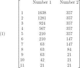
  . The following table displays the results of modulo .
The above table indicates that to get  , the power can stop at
  , one less than the modulus. According to Fermat’s theorem, this is always the case as long as the modulus is a prime number and as long as the base is a number that is not divisible by the modulus.
___________________________________________________________________________________________________________________
Fermat’s Little Theorem
The following is a statement of the theorem.
Theorem 1 (Fermat’s Little Theorem)
If is a prime number, then  for any integer with
  .
.
Note that  refers to the greatest common divisor of the integers and
  . When
  , the integers and are said to be relatively prime. We also use the notation
  to mean that the integer divides without leaving a remainder.
In the discussion at the end of the above example, the base is a number that is required to be not divisible by the modulus . If the modulus is a prime number, is a number that is not divisible by the modulus is equivalent to the condition . See the section called Variations below.
We will present below a formal proof of the theorem. The following example will make the idea of the proof clear. Let . Let  . Calculate the following numbers:
For each of the above numbers, find the least residue modulo . The following shows the results.
The above calculation shows that the least residues of  are just an rearrangement of
  . So we have:
Because  (10 factorial) is relatively prime with , we can cancel it out on both side of the congruence equation. Thus we have
  for .
for .
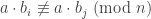
The above example has all the elements of the proof that we will present below. The basic idea is that whenever and the modulus are relatively prime, taking the least residues of  modulo produces the numbers
  (possibly in a different order).
We have the following lemma.
Lemma 2
Let be a prime number. Let be a positive integer that is relatively prime with , i.e., . Then calculating the least residues of the number modulo gives the numbers .
Proof of Lemma 2
Let  be the least residues of modulo . That is, for each
  ,
,  is the number with
  such that
  . Our goal is to show that are the numbers . To this end, we need to show that each satisfies
  and that the numbers are distinct.
First of all,  . Suppose
  . Then
  and
and  . By Euclid’s lemma, either
  or
or  . Since ,
  . So . But is a positive integer less than . So we have a contradiction. Thus each satisfies .
Now we show the numbers are distinct (the list has exactly  numbers). To this end, we need to show that
  when
when  . Suppose we have
  and . . Then
  . Since and are relatively prime, there is a cancelation law that allows us to cancel out on both sides. Then we have
  . This means that
  . Since
  and are positive integers less than the modulus , for to happen, must equals , contradicting . It follows that are distinct.
Taking stock of what we have so far, we have shown that  . Both sides of the set inclusion have distinct numbers. So both sides of the set inclusion must equal.
We now prove Fermat’s little theorem.
Proof of Theorem 1
Let be a prime number. Let be a positive integer such that . By Lemma 2, the least resides of modulo are the numbers . Thus we have the following congruence equations:
Just as in the earlier example, we can cancel out  on both sides of the last congruence equation. Thus we have .
___________________________________________________________________________________________________________________
Variations
There are several ways to state the Fermat’s little theorem.
Theorem 3
If is a prime number, then  for any integer .
Theorem 3 is a version of the Fermat’s theorem that is sometimes stated instead of Theorem 1. It has the advantage of being valid for all integers without having the need to consider whether and the modulus are relatively prime. It is easy to see that Theorem 3 implies Theorem 1. On the other hand, Theorem 3 is a corollary of Theorem 1.
To see that Theorem 3 follows from Theorem 1, let be prime and be any integer. Suppose and the modulus are not relatively prime. Then they have a common divisor  . Since is prime,
  must be . So is an integer multiple of . Thus divides both and any power of . We have
  for any integer . In particular, . The case that and the modulus are relatively prime follows from Theorem 1.
We now consider again the versions that deal with  . The following is a side-by-side comparison of Theorem 1 with another statement of the Fermat’s little theorem. Theorem 1 is re-labeled as Theorem 4a.
Theorem 4a (= Theorem 1)
If is a prime number, then for any integer with .
Theorem 4b
If is a prime number, then for any integer that is not divisible by .
The equivalence of these two versions follows from the fact that for any prime number , if and only if is not divisible by . It is straightforward to see that if , then is not divisible by . For the converse to be true, must be a prime number.
Since any integer is congruent modulo to some with  , the following version is also an equivalent statement of the Fermat’s little theorem.
Theorem 4c
If is a prime number, then for any integer such that .
___________________________________________________________________________________________________________________
The Converse
It is a natural question to ask whether the converse of the Fermat’s little theorem is true. In many sources, it is stated that the converse is not true. It turns out that the answer depends on the versions. The converse of Theorem 4a is not true, while the converse of Theorem 4b and the converse of Theorem 4c are true. Let’s compare the following statements about the positive integer :
Statement (1) is the conclusion of Theorem 4a, while statement (2) is the conclusion of Theorem 4b.
The statement (2) is a stronger statement. Any positive integer that satisfies (2) would satisfy (1). This is because the set of all integers for which is a subset of the set of all integers for which is not divisible by .
However, statement (1) does not imply statement (2). Any composite positive integer that satisfies (1) is said to be a Carmichael number. Thus any Carmichael number would be an example showing that the converse of Theorem 4a is not true. There are infinitely many Carmichael numbers, the smallest of which is  . See the blog post Introducing Carmichael numbers for a more detailed discussion.
Any positive integer satisfying statement (2) is a prime number. Thus the converse of Theorem 4b is true. We have the following theorem.
Theorem 5
Let be an integer with  . Then is a prime number if and only if statement (2) holds.
Proof of Theorem 5
The direction  is Theorem 4b. To show
  , we show the contrapositive, that is, if is not a prime number, then statement (2) does not hold, i.e., there is some not divisible by such that
  .
.
Suppose is not prime. Then has a divisor where  . We claim that . By way of a contradiction, suppose . Then
  . Since
  , we have
  . So
. So  for some integer . Now we have
  . This implies that divides
  . This is impossible since
  . This establishes the direction .
As a Carmichael number,  satisfies statement (1). However it would not satisfy statement (2). By the proof of Theorem 5, if is a prime factor of , then
  . Note that
  since
since  is a divisor of . In fact,
  and
and  . We also have
  . Thus statement (1) is a weaker statement.
Any statement for the Fermat’s little theorem can be used as a primality test (Theorems 4a, 4b or 4c). On the face of it, Theorem 5 seems like an improvement over Theorem 4a, 4b or 4c since Theorem 5 can go both directions. However, using it to show that is prime would require checking for all with  . If has hundreds of digits, this would be a monumental undertaking! Thus this primality test has its limitation both in terms of practical considerations and the possibility of producing false positives.
__________________________________________________________________________________________________________________


such that
.
for some positive integer


and
for each


 where
where  (see Example 3 below).
 . Solving it means finding all integers
  or
or  for some integer
  is a solution. After one solution is found, there are infinitely many other solutions. For this example, they are
  for all integers
  . Are there other solutions that are not congruent to
  and
and  . Any solution to
  , we can simply narrow our focus by looking for solutions only among the least residues.
 with
with  .
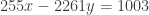
. is another way of stating the linear congruence
  .
. . So they both have the same solutions. So we focus on solving
  . We carry out the Euclidean algorithm.


 . Note that
  . So the equation
  . We work backward in the steps of the Euclidean algorithm as follows:
 , we have
  . Thus the number pair
  and
and  is a particular solution of the equation

 is any integer.
 . The solutions are
  for
for  . Note that the number of solutions is identical to the GCD of
  and the modulus
  .
. .
. . For the same reason, the equation
  has no solutions.
 .
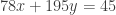
. . We apply the Euclidean algorithm.


 . With Example 1 as a guide, there is only one solution to the given linear congruence.
 . So
. So  is a particular solution to the given linear congruence equation and its corresponding linear Diophantine equation
  .
. for any integer
  where
where  .
.  , the product of
  and
and  where
where  and
and  are prime numbers. The number
  and
and  is an example for an encryption key for the RSA algorithm. Finding the decryption key entails solving the linear congruence
  .
. . This will lead to a particular solution to the equation
  be a solution to the linear congruence equation
  where
where 
 for some integer
  . Thus the number pair
  is a particular solution to the linear Diophantine equation


 where
where  . By the division algorithm, we have
  for some integer
  and some integer
  . Now, we have the following calculation:
 . By the division algorithm, we have
  for some integer
  . We have the following calculation.

 is one of the numbers in (2). So the


 . So by a solution to
  that satisfies the equation.
 are integers, the first step is to find the greatest common divisor of
  . The equation
  always has a solution. In fact this statement is called the extended Euclidean algorithm. The solution can be obtained by working backward from the Euclidean algorithm (when we use it to obtain the GCD).
 . We can trace back the steps in finding the GCD to see that
  .
.
 and
and  is a solution to the equation
  . Based on this development, we can see that
 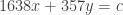 always has a solution as long as
  . For example, the equation
  .
.
 and
and  is a solution to the equation
  .
. for some integer
  indicates that the pair
  and
and  is a solution to
  and
and 
 . On the other hand, if we decrease
  . The net effect is that the left-hand side of the equation remains unchanged.
 and
and 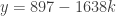 for all integers
  and
and  is also a solution to the equation


 and
and  is a solution to the equation


 . Note that after canceling out all the common prime factors of two numbers, the resulting two numbers should be relatively prime.
 divides
  . Because
  . So the number
  . So for some integer
 into (1), we have
  . This leads to the following.
 and
and  (the negative sign of


 , which divides
  . So the equation has solutions. We need to find a specific solution. First we work backward from the above divisions to find a solution to
  . Then we multiply that solution by
  . Working backward, we get:
 and
and  is a solution of
  and
and  is a solution of
  .
.

 , note that the GCD of
  and
and  is
is  , which does not divide
  . Thus the equation has no solutions.
 and
and  . We apply the Euclidean algorithm.


 and
and  is a specific solution to


 , then we have conclusive proof that
  .
. . If it is greater than 1, then stop and output
  .
. , then
  and such that
  , then the integer
  for all
  probability that the Fermat test will not detect the compositeness of the composite number
  and such that
  , which is derived as follows:
 .
. , then we are done. So assume that
  enumerate all bases to which
  for all
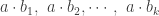
 for
for  is defined to be the number of integers
  many bases in the interval
 modulo
  and the modulus
  . The naïve approach is to compute by repeatedly multiplying by
  modulo
  .
.
 multiplications and then
  and instead is an integer with hundreds or even thousands of digits.
 modulo

 . The calculation in (3) is the step that gives the word “multiply” in the name “square-and-multiply”. In this step, we multiply the results obtained from the previous step.
 , use the following steps. The following steps correspond with the steps in the above example.
 or
or  . In particular, we assume that
  .
. , compute
  modulo
  . We arrange the calculation in the following table.
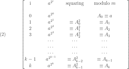

 many be zero. Step (3) also requires at most
  multiplications and
  . Take natural log of both sides, we have
  and
and 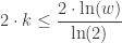 . So the fast powering algorithm requires at most
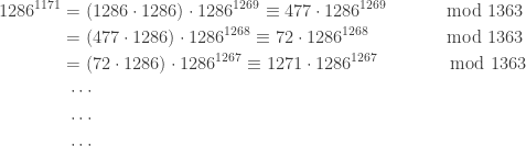
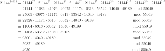
 , which is a Mersenne prime, which has 39 digits. Now
  . By the above calculation, the fast powering algorithm would take at most 254 multiplications and at most 254 divisions to do the power congruence computation.

 is a prime number. So
  . Thus we have:
 are:
are:
 modulo
 .
.
 has 155 digits and has the following three prime factors:


 for some positive integers
  of all positive integer divisors of
  be the least element of
  . Suppose the lemma is true for all positive integers
  .
. , then
  or
or  .
. , then
  for some
  . Suppose that
  . By Euclid’s lemma, we have
  . In the first case, the induction hypothesis tells us that
  . In the second case
  .
. and since the lemma is true for
  and
and  as the same factorization for the integer
  .
. and
and  are prime factorizations of the integer
  is identical to some
  and each
  is identical to some
  . This implies that the prime numbers
  are simply a rearrangement of
  such that the only difference for the two factorizations is in the order of the factors.
  . Thus
  divides
  , or we write
  . By Lemma 3,
  for some
  . Then cancel out
 divides the right-hand side of the above equation. By Lemma 3,
  for some
  . Otherwise, there would be some
  . Thus we have
  and that the two factorizations are really just rearrangement of each other.
 . Such representation of an integer is called a prime-power decomposition. For example,
  .
. and
and  , then
  . Multiplying both sides by
 , which implies that
  . If
. If  ,
,  , which implies that
  and
and  .
. to its lowest terms. The first step is to factor each of the numerator and denominator using their prime factors.
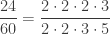

 , which is the greatest common divisor of 24 and 60.
 . In other words,
  and
and  . When
  .
. and
and  .
. and
and  , then
  .
. .
. 
 .
. , then
  .
. and
and  .
. and
and  , we have
  . Since
  and
and  .
.

 . To go from row 2 to row 3, divide the larger number
  . Repeat the process until one of reaching the remainder of zero. Then the other number in the last row is the greatest common divisor. The following is the same algorithm with the divisions added.
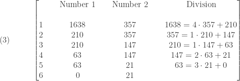
 and
and  be positive integers. Assume
  . Start with the pair
  and forms a new pair that consists of the smaller number and the remainder derived from dividing the larger number by the smaller. The process stops when reaching a remainder of zero. Then the other number in the last pair is the GCD of


 where the remainder
  . We have
  where
where  is the GCD of the original pair
  must stop at some point. Eventually
  . Then
  .
.

 and
and  . The following shows the divisions used in Table (3) above.


 . Note that
  . Let
. Let  be the following subset of
 for some positive integer
  . If
. If  ,
,  , which is less than
  and
and  such that
 . Since
  and
and  ,
,  . This means that
  , since both
  and in turns
  .
.  means that
  (in words, we say
  for a unique integer
  .
. , clearly
  . We can assume that
  .
. . By the division algorithm, there are integers
  where
where  . Thus
  . By the division algorithm, there are integers
  where
where  . Thus
  . Note that
  . Thus
  /
/